Overview
- Every day I receive data about total U.S. sales, which is computed in a cell as the sum of East, North, and South region sales. How can I extract East, North, and South sales to separate cells?
- I download quarterly gross national product (GNP) data from the
Web. The cell containing first quarter data for 1980 contains the entry 1980.1 5028.8. How can I place the date and GNP value in different cells?
- In the spreadsheet I use for a mailing list, column A contains people's names, column B contains their street address, and column C contains their city and zip code. How can I create each person's full address in column E?
When someone sends you data or you download data from the Web, often the data isn't formatted the way you want. For example, when downloading sales data, dates and sales amounts might be in the same cell but you need them to be in separate cells. How can you manipulate data so that it has the format you need? The answer is to become good at using Excel's set of text functions. In this chapter, I'll show you how to use the following Excel text functions to magically manipulate your data until it looks the way you want:
- LEFT
- RIGHT
- MID
- TRIM
- LEN
- FIND
- SEARCH
- CONCATENATE
- REPLACE
- VALUE
Text Function Syntax
The file Reggie.xls, shown in Figure 6-1, includes examples of text functions. You'll see how to apply these functions to a specific problem later in the chapter, but let's begin by describing what each of the text functions do. Then we'll combine these functions to perform some fairly complex manipulations of data.
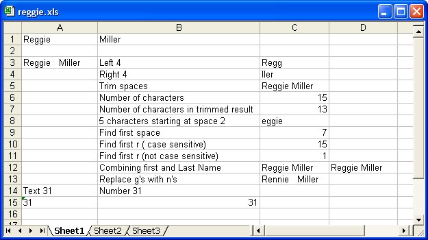
Figure 6-1: Examples of text functions.
The RIGHT Function
The function RIGHT(text,k) returns the last k characters in a text string. For example, in cell C4, the formula RIGHT(A3,4) returns ller.
The MID Function
The function MID(text, k, m) begins at character k of a text string and returns the next m characters. For example, the formula MID(A3,2,5) in cell C8 returns characters 2-6 from cell A3, the result being eggie.
The TRIM Function
The function TRIM(text) removes all spaces from a text string except for single spaces between words. For example, in cell C5 the formula TRIM(A3) eliminates two of the three spaces between Reggie and Miller and yields Reggie Miller.
The LEN Function
The function LEN(text) returns the number of characters in a text string (spaces are included). For example, in cell C6 the formula LEN(A3) returns 15 because cell A3 contains 15 characters. In cell C7, the formula LEN(C5) returns 13. Because the trimmed result in cell C5 has two spaces removed, cell C5 contains two less characters than the original text in A3.
The FIND and SEARCH Functions
The function FIND(text to find, actual text, k) returns the location at or after character k of the first character of text to find in actual text. FIND is case sensitive. SEARCH has the same syntax as FIND, but it is not case sensitive. For example, if we enter FIND ("r",A3,1) in cell C10, Excel returns 15, the location of the first lowercase r in the text string Reggie Miller. (The uppercase R is ignored because FIND is case sensitive.) Entering SEARCH("r",A3,1) in cell C11 returns 1 because SEARCH matches r to either a lowercase or an uppercase character. Entering FIND(" ",A3,1) in cell C9 returns 7 because the first space in the string Reggie Miller is the seventh character.
CONCATENATE and & Functions
The function CONCATENATE(text1, text2, . . ., text30) can be used to join up to 30 text strings into a single string. The & operator can be used instead of CONCATENATE. For example, entering in cell C12 the formula A1&" "& B1 returns Reggie Miller. Entering in cell D12 the formula CONCATENATE(A1," ",B1) yields the same result.
REPLACE Function
The function REPLACE(oldtext, k,m, newtext) begins at character k of oldtext and replaces the next m characters with newtext. For example, in cell C13 the formula REPLACE(A3,3,2,"nn") replaces the third and fourth characters ( gg) in cell A3 with nn. This formula yields Rennie Miller.
VALUE Function
The function VALUE(text) converts a text string that represents a number to a number. For example, entering in cell B15 the formula VALUE(A15) converts the text string 31 in cell A15 to the numerical value 31. You can tell that the value 31 in cell A15 is text because it is left-justified. Similarly, you can tell that the value 31 in cell B15 is a number because it is right-justified.
Text Functions in Action
You can see the power of text functions by using them to solve some actual problems that were sent to me by former students working in Fortune 500 corporations. The key to solving each problem is to combine multiple text functions in a single formula.
I have a spreadsheet in which each cell contains a product description, a product ID, and a product price. How can I put all the product descriptions in column A, all the product IDs in column B, and all the prices in column C?
In this example, the product ID is always defined by the first 12 characters and the price is always indicated in the last 8 characters (with two spaces following the end of each price). Our solution, contained in the file Lenora.xls and shown in Figure 6-2, uses the LEFT, RIGHT, MID, VALUE, TRIM, and LEN functions.

Figure 6-2: Use the TRIM function to trim away excess spaces.
It's always a good idea to begin by trimming excess spaces, which we do by copying from B4 to B5:B12 the formula TRIM(A4). The only excess spaces in column A turn out to be the two spaces inserted after each price. The results of using the TRIM function are shown in Figure 6-2.
To capture the product ID, we need to extract the 12 leftmost characters from column B. We copy from C4 to C5:C13 the formula LEFT(B4,12). This formula extracts the 12 leftmost characters from the text in cell B4 and the following cells, yielding the product ID, as you can see Figure 6-3.

Figure 6-3: Text functions extract the product ID, price, and product description from a single text string.
To extract the product price, we first note that the price occupies the last 6 digits of each cell, so we need to extract the rightmost 6 characters in each cell. I copy from cell D4 to D5:D12 the formula VALUE(RIGHT(B4,6). I use the Value function to turn the extracted text into a numerical value. Without converting the text to a numerical value, you couldn't perform mathematical operations on the prices.
Extracting the product description is much trickier. By examining the data, we can see that if we begin our extraction with the 13th character and continue until we are 6 characters from the end of the cell, we will have the data we want. Copying the following formula from E4 to E5:E12 does the job: MID(B4,13,LEN(B4)-6-12). Len(B4) returns the total number of characters in the trimmed text. This formula ( MID for Middle) begins with the 13th character and then extracts the number of characters equal to the total number less the 12 characters at the beginning (the product ID) and the 6 characters at the end (price). This subtraction simply leaves the product description!
Now suppose we are given the data with product ID in column C, the price in column D, and the product description in column E. Can we put these values together to recover our original text?
Text can easily be combined by using the CONCATENATE formula. Copying-from F4 to F5:F12 the formula CONCATENATE(C4," ",E4," ",D4) recovers our original (trimmed) text, which you can see in Figure 6-4.

Figure 6-4: Using concatenation to recombine product ID, product description, and price.
The concatenation formula starts with the product ID in cell C4. The empty quotation marks (" ") insert a space. Next we add the product description from cell E4 and another space. Finally, we add the price from cell D4. We have now recovered the entire text describing each computer! Concatenation can also be performed by using the & sign. We could also recover the original product ID, product description, and price in a single cell with the formula C4&" "& E4&" "& D4.
If the product IDs did not always contain 12 characters, this method of extracting the information would fail. We could, however, extract the product IDs by using the FIND function to discover the location of the first space. Then we could obtain the product ID by using the LEFT function to extract all characters to the left of the first space. The example in the next section will show how this approach works.
If the price did not always contain precisely six characters, extracting the price would be a little tricky. You would need to use the OFFSET function, which you will learn about in Chapter 21.
Every day I receive data about total U.S. sales, which is computed in a cell as the sum of East, North, and South region sales. How can I extract East, North, and South sales to separate cells?
This problem was sent to me by an employee in Microsoft's finance department. She received a spreadsheet each day containing formulas such as =50+200+400, =5+124+1025, and so on. She needed to extract each number into a cell in its own column. For example, she wanted to extract the first number (East sales) in each cell to column C, the second number (North sales) to column D, and the third number (South sales) to column E. What makes this problem challenging is that we don't know the exact location of the character at which the second and third numbers start in each cell. In the first cell in our example, the second number begins with the fourth character. In the second cell, the second number begins with the third character. The data we're using in this example is in the file SalesStripping.xls, shown in Figure 6-5. By combining the FIND, LEFT, LEN, and MID functions, we can easily solve this problem as follows:
- Use the Edit, Replace command to replace each equal sign with a space. This converts each formula into text.
- Use the FIND function to locate the two plus (+) signs in each cell.
- East sales are represented by every character to the left of the first plus sign.
- North sales are represented by every character between the first and second plus sign.
- South sales are represented by every character to right of the second plus sign.

We begin by finding the location of the first plus sign for each piece of data. By copying from B3 to B4:B6 the formula FIND("+",A3,1), we can locate the first plus sign for each data point. To find the second plus sign, we begin one character after the first plus sign, copying from C3 to C4:C6 the formula FIND("+",A3,B3+1).
To find East sales, we use the LEFT function to extract all the characters to the left of the first plus sign, copying from D3 to D4:D6 the formula LEFT(A3,B3-1). To extract the North sales, we use the MID function to extract all the characters between the two plus signs. We begin one character after the first plus sign and extract the number of characters equal to (Position of 2nd plus sign)-(Position of 1st plus sign) - 1. If you leave out the -1, you'll get the second + sign. (Go ahead and check this.) So, to get the North sales, we copy from E3 to E4:E6 the formula MID(A3,B3+1,C3-B3-1).
To extract South sales, we use the RIGHT function to extract all the characters to the right of the second plus sign. South sales will have the number of characters equal to (Total characters in cell) - (Position of 2nd plus sign). We compute the total number of characters in each cell by copying from F3 to F4:F6 the formula LEN(A3). Finally, we obtain South sales by copying from G3 to G4:G6 the formula RIGHT(A3,F3-C3).
Using the Text To Columns Command to Extract Data
There is an easy way to extract East, North, and South sales (and data similar to this example) without using text functions. Simply select cells A3:A6, and then choose Text To Columns on the Data menu. Select Delimited, click Next, and then fill in the dialog box shown here:


No comments:
Post a Comment