Chapter 1: Range Names

Overview

• I want to add up sales in Arizona, California, Montana, New York, and New Jersey. Can I use a formula to compute total sales in a form such as AZ+CA+MT+NY+NJ instead of SUM(A21:A25) and still get the right answer?
• To compute total sales for a year, I often average the 12 monthly sales below the current cell. Can I name my formula annualaverage so that when I enter annualaverage in a cell the appropriate average is computed?
• How can I easily select a cell range?
• How can I paste a list of all range names (and the cells they represent) into my spreadsheet?

You have probably received spreadsheets that use formulas such as SUM(A5000:A5049). Then you have to struggle to understand what's contained in cells A5000:A5049. If cells A5000:A5049 contain sales in each U.S. state, wouldn't the spreadsheet be easier to understand if the formula was SUM(USSales)? In this chapter, I'll teach you how to name individual cells, ranges of cells, constants, and formulas. I'll also show you how to use range names in formulas.

How Can I Create Range Names?

There are three ways to create range names:

• Entering a range name in the Name box
• Choosing the Name, Create command from the Insert menu
• Choosing the Name, Define command from the Insert menu

Using the Name Box to Create a Range Name

The Name box is located directly above the label for column A, as you can see in Figure 1-1. (To see the Name box, you need to display the Formula bar.) To create a range name using the Name box, simply select with the mouse the cell or range of cells that you want to name, click in the Name box, and then type the range name you want to use. Press Enter, and you've created the range name. Clicking on the drop-down arrow for the Name box displays the range names defined in the current workbook. You can also display all the range names in a workbook by pressing the F3 button, which displays the Paste Name dialog box. When you select a range name from the Name box, Excel selects the cells corresponding to that range name. This enables you to check that you've chosen the cell or range that you intended to.

Figure 1-1: You can create a range name by selecting the cell range you want to name and then typing the range name in the Name box.

Creating Range Names by Using the Name Create Command

The spreadsheet States.xls contains sales during March for each of the 50 U.S. states. Figure 1-2 shows a subset of this data. We would like to name each cell in the range B6:B55 with the correct state abbreviation. To do this, select the range A6:B55, choose Insert, Name Create, and then choose the Create Names In Left Column option, as indicated in Figure 1-3.

 Figure 1-2: By naming the cells that contain state sales with state abbreviations, you can use the abbreviation when you refer to the cell rather than the cell's column and row number.

Figure 1-3: Use the Name, Create command on the Insert menu to name cell ranges. The Create Names dialog box provides options for naming cell ranges.

Excel now knows to associate the names in the left column of the selected range with the cells in the second column of the selected range. Thus B6 is assigned the range name AL, B7 is named AK, and so on. Note that creating these range names in the Name box would have been incredibly tedious! Click on the drop-down arrow in the Name box if you don't believe that these range names have been created.

Creating Range Names by Using the Name Define Command

If you choose the Insert, Name Define command, the dialog box shown in Figure 1-4 comes up.

Figure 1-4: The Define Name dialog box before creating any range names.

Suppose you want to assign the name range1 (range names are not case sensitive) to the cell range A2:B7. Simply type range1 in the Names In Workbook box and then go down to the Refers To area and point to the range or type in =A2:B7. Click Add, and you're done. The Define Name dialog box will now look like Figure 1-5.

Figure 1-5: Define Name dialog box after creating a range name.

Of course, if you now click in the Name box, the name range1 will appear. Now let's look at some specific examples of how to use range names.

I want to add up sales in Arizona, California, Montana, New York, and New Jersey. Can I use a formula to compute total sales in a form such as AZ+ CA+ MT+ NY+ NJ instead of SUM(A21:A25) and still get the right answer?

Let's return to the file States.xls in which we assigned each state's abbreviation as the range name for the state's sales. If we want to compute total sales in Alabama, Alaska, Arizona, and Arkansas, we could clearly use the formula SUM(B6:B9). We could also point to cells B6, B7, B8, and B9, and the formula would be entered as =AL+AK+AZ+AR. The latter formula is, of course, much easier to understand.

As another illustration of how to use range names, look at the file HistoricalInvest.xls, shown in Figure 1-6, which contains annual percentage returns on stocks, T-Bills, and bonds. (The rows for years 1935-1996 are hidden.)



Figure 1-6: Historical investment data.

After selecting the cell range B7:D81 and choosing Insert, Name Create, we choose to create names in the top row of the range. The range B8:B81 is named Stocks, the range C8:C81 T.Bills, and the range D8:D81 T.Bonds. Now we no longer need to remember where our data is. For example, in cell B84, after typing =AVERAGE(, we can press F3 and the Paste Name dialog box appears, as shown in Figure 1-7.



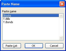
Figure 1-7: You can add a range name to a formula by using the Paste Name dialog box.
Then we can select Stocks in the Paste Name list and click OK. After enteringthe closing parentheses, our formula, =AVERAGE(Stocks), computes the average return on stocks (12.05 percent). The beauty of this approach is that even if we don't remember where the data is, we can work with the stock return data anywhere in the workbook!

If we use a column name (in the form A:A, C:C, and so on) in a formula, Excel treats an entire column as a range name. For example, entering the formula =AVERAGE(A:A) will average all numbers in column A. Using a range name for an entire column is very helpful if you frequently enter new data into a column. For example, if column A contains monthly sales of a product, as new sales data is entered each month, our formula always computes an uptodate monthly sales average. I caution you, however, that if you enter the formula =AVERAGE(A:A) in column A, you will get a circular reference message because the value of the cell containing the average formula depends on the cell containing the average. You will learn how to resolve circular references later in the book, in Chapter 11.

How Do I Delete a Range Name?

To delete a range name, simply choose Insert, Name Define to bring up the Define Name dialog box. (See Figure 1-5.) Select the range name you want to delete, and then click Delete. Unfortunately, Excel lets you delete only one range name at a time.

How Do I Change a Range Name?

To change a range name, select Insert, Name Define to bring up the Define Name dialog box. (See Figure 1-5.) Select the range whose name you want to change, and then enter a new name or the cell range to which the range name refers. You can change the range by typing in the new range or by selecting the new range in the worksheet. Click OK, and the range is changed.

How Do I Name a Constant?

In many spreadsheets a value occurs so often that you might want to name it to use it as a constant. For example, suppose sales during the current year are $10 million and sales are growing 10 percent a year. (See the file Growth.xls.) We can name the annual growth rate Growth by choosing Insert, Name Define, filling in the Names In Workbook box and the Refers To area as shown in Figure 1-8, and then clicking OK.


Figure 1-8: You can name a value that occurs frequently in a workbook and use it as a constant.

Now everywhere in your spreadsheet, Growth will be interpreted as 1.1.

If you haven't already, open the file Growth.xls. Copying from F11 to G11:H11 the formula E11*Growth generates the sales for years 1-6 that grow at 10 percent a year, as you can see in Figure 1-9.


Figure 1-9: Sales growth was calculated using a named constant.

To compute total sales for a year, I often average the 12 monthly sales below the current cell. Can I name my formula annual average so that when I enter annual average in a cell the appropriate average is computed?

Often you perform the same type of operation over and over. Wouldn't it be nice if you could name the formula that performs the operation? Then, whenever you needed to use the formula, you could call up the formula from the Paste Name dialog box. Here's an example.

Suppose that we repeatedly average 12 cells below the current cell to compute average monthly sales for several products during a calendar year. (See the file Sales.xls and Figure 1-10.) We would like to start 2 rows below the current cell and average 12 cells to get an average of monthly sales. To name this operation, we begin by going to any cell. I used cell B2 in this example. Choose Insert, Name Define to bring up the Define Name dialog box. Select the name annualaverage, and then look at the Refers To area, as indicated in Figure 1-11.


Figure 1-10: Data for naming a formula to average 12 months of sales.



Figure 1-11: Naming a formula to average 12 months of sales.

You enter the formula that performs the operation given the current cell location. Because we are in cell B2, we want to average cells B4:B15, so we enter the formula =AVERAGE(B4:B15). You must type in the formula you want rather than enter the formula by pointing. Now, if we enter the name annualaverage in any cell, the formula will drop down 2 cells and average the next 12 cells below the current cell. To illustrate how this named formula works, I've entered the formula =annual average in cells C2:E2. You now obtain the annual average of sales for products 2-4. Note that if you are in cell E2 and you select Insert, Name Define, the Refers To area indicates that the range annualaverage refers to the formula =Average(E4:E15), which is the correct formula!

How can I easily select a cell range?

If you have selected a cell within a cell range, press Ctrl+Shift+* to select the entire range.

How can I paste a list of all range names (and the cells they represent) into my spreadsheet?

Press F3 to display the Paste Name box, and then click the Paste List button. A list of range names and the cells each corresponds to will be pasted into your spreadsheet, beginning at the current cell location.

Remarks

• Excel does not allow you to use the letters r and c as range names. Instead it will create a range name r_ or c_.
• If you use Insert, Name Create to create a range name and your name contains spaces, Excel inserts an underscore (_) to fill in the spaces. For example, the name Product 1 is created as Product_1.
• Range names cannot begin with numbers or look like a cell reference. For example, 3Q or A4 are not allowed as range names.
• The only symbols allowed in range names are periods (.) and underscores (_).